Demand Forecasting in Manufacturing – Process, Methods, and Tools for SMEs

Demand forecasting done right makes the difference between reactive and structured decision-making. It gives purchasing, inventory management, and production planning teams more time to prepare and takes a lot of guesswork out of replenishment decisions.

Key takeaways

• Demand forecasting is the process of estimating future customer demand using historical data, business information, market knowledge, and various forecasting methods. In manufacturing, it primarily helps predict which products will be needed, in what quantities, and when.
• Demand forecasting supports different manufacturing models in different ways. Make-to-stock companies use it heavily for finished-goods planning, while make-to-order and assemble-to-order manufacturers can use it to prepare materials, subassemblies, and capacity.
• There is no single best forecasting method. Historical and moving averages, trend and seasonal models, exponential smoothing, causal models, and judgment-based forecasting each suit different demand patterns and data situations.
• A useful forecast starts with the planning decision it needs to support. Set an appropriate horizon, prepare the demand data, identify demand patterns, create a baseline forecast, and adjust it when reliable new business information becomes available.
• Forecast accuracy should be measured and improved over time. Compare forecasts with actual demand and simple baselines, track metrics such as MAE, MAPE, WAPE, and forecast bias, and check whether manual overrides genuinely improve results.
• Forecasting creates the most value when it’s connected with operational planning. Manufacturing ERP and MRP systems can link expected demand with inventory, master production scheduling, material requirements, purchasing, and production capacity.

What is demand forecasting in manufacturing?

Demand forecasting is the process of estimating future customer demand using historical data, current business information, market knowledge, and statistical or software-assisted forecasting methods. In manufacturing, the focus is generally on the quantities of finished products customers are expected to require over a defined period.

The focus on quantities is an important distinction. Financial sales forecasts might predict that revenue will increase by 10%, but that figure alone doesn’t tell purchasing which materials to order or production which products to make. Manufacturing relies on this information above all to know which products are likely to be required, in what quantities, and ideally, by when.

A product demand forecast isn’t a promise that a particular quantity will be sold. It’s an informed planning estimate that reduces uncertainty enough to enable a company to make better decisions about inventory management, production, suppliers, capacity, and cash flow.

Forecasting doesn’t eliminate risk altogether, though. Well-prepared forecasts can still be disrupted by cancellations, supplier problems, economic shocks, new competitors, or unexpected shifts in product demand. The idea is to give companies a more useful starting point than intuitive guesswork or purely reactive planning.

Demand forecasting vs. demand planning vs. demand management

Demand forecasting, demand planning, and demand management are closely related but address different aspects of the planning process.

• Demand forecasting estimates what customers are likely to require. Its main output is an expected quantity, value, or range for a future period.
• Demand planning turns the forecast into an agreed demand plan by reviewing it against current business information, customer knowledge, market activity, and commercial priorities.
• Demand management is the broader process of monitoring, prioritizing, influencing, and responding to demand across sales, marketing, operations, purchasing, and finance.

The exact use of these terms varies between companies and software providers. In practice, forecasting produces the initial estimate, while demand planners and demand management are more concerned with what the company should do with it.

Why demand forecasting matters in manufacturing and distribution

Most manufacturers and distributors need to commit resources before demand becomes certain in the form of incoming orders. Materials take time to arrive, some suppliers impose minimum order quantities (MOQs), and production capacity may be tied up with prior orders.

A demand forecast gives you visibility into what may be required sooner. That helps reduce stockouts and overproduction, order long-lead materials earlier, prepare production capacity for expected peaks, etc. The operational value comes from connecting expected demand with supply decisions. But that only works if the forecast is reliable.

Demand forecasting in make-to-stock manufacturing

Make-to-stock (MTS) manufacturers produce finished goods in anticipation of demand. Companies like this typically rely most heavily on demand forecasting because production takes place before firm customer demand is known.

If demand is underforecasted, you might run out of goods, thereby losing sales, damaging customer satisfaction, failing to meet distributor agreements, and potentially incurring overtime or expediting costs. If it’s overforecasted, you end up tying up cash in excess inventory that may need to be discounted, reworked, or written off.

Demand forecasting is especially important in MTS environments because expected demand is a major input to the master production schedule (MPS), a longer-term production planning tool that helps determine what should be produced, in what quantities, and during which periods.

Demand forecasting in make-to-order and assemble-to-order manufacturing

Make-to-order (MTO) and assemble-to-order (ATO) manufacturers generally avoid producing finished goods until a customer order confirms demand. This reduces the need to forecast finished-product inventory size, but that doesn’t make demand forecasting irrelevant. An MTO or ATO manufacturer may still need to prepare common raw materials, prefabricate longer lead-time subassemblies, or account for workstation constraints.

Suppose you manufacture customizable industrial control panels. You don’t know the configuration of each panel that’ll be ordered, but your data from past orders is still useful for sourcing relevant PCBs, power supplies, buttons, or assemblies to speed up delivery times.

Forecasts in MTO/ATO environments should be handled carefully, though. They provide an early signal for materials and shared resources that would otherwise be difficult to secure at short notice. But that doesn’t mean you should treat uncertain demand as a go-ahead to build highly customized finished products.

Demand forecasting for distributors and wholesalers

For distributors and wholesalers that don’t produce in-house goods, demand forecasting is tied to replenishment and inventory allocation. They need enough stock to meet customer demand but also to avoid overinvesting in slow-moving or unpredictable products.

This challenge grows as the number of stock keeping units (SKUs) you offer increases. A distributor may simultaneously manage fast-moving standard items, seasonal products, specialist spare parts, and new items with little sales history. Using the same replenishment logic for all these creates significant inventory problems.

Forecasts can help distributors prepare for expected seasonal demand, plan purchases before supplier constraints arise, identify products at risk of running short, and avoid accumulating too much slow-moving stock.

Types of demand forecasting

Demand forecasts can be classified in several ways. For an SME, the most useful distinctions concern where the information comes from and how far into the future the forecast looks.

Qualitative, quantitative, and hybrid forecasting

Qualitative demand forecasting

Qualitative forecasting relies mostly on business judgment rather than mathematical analysis of historical demand. Information can come from a sales force composite, customers, distributors, management, market research, or industry specialists. It’s a useful approach when historical demand is unavailable, like for new products, or when consumer behavior and market trends are rapidly changing or a major regulatory change is expected.

Judgmental forecasting can help respond quickly to information that hasn’t yet appeared in data. Its weakness is subjectivity – salespeople may be overly optimistic about potential deals, product teams may overestimate the success of a launch, and managers may unintentionally adjust forecasts toward internal targets.

Systematic approaches like structured assumptions, documenting outcomes, and clear ownership make qualitative forecasts more useful and easier to evaluate.

Quantitative demand forecasting

Quantitative forecasting uses historical sales data and statistical methods to estimate future demand. This is done using inputs like customer order quantities, shipments, historical consumption, prices, promotions, and other directly measurable demand signals.

Quantitative forecasting works well when the company has consistent historical records and recurring sales. Its limitation is that historical data only describes what has already happened. A model based solely on historical demand won’t know when a customer is planning a major order, whether a product will soon be discontinued, or whether a previous spike actually resulted from a one-time project – at least not unless that data is taken into account in the model.

Hybrid demand forecasting

A practical third option is hybrid forecasting, which combines a quantitative baseline with structured human judgment. The system or analyst creates an initial forecast from historical data, after which employees review and adjust it using current business information. For many SMEs, this is the go-to option. It gives the business an evidence-based starting point while still allowing decision-makers to account for information that historical data doesn’t contain.

You may also encounter the terms passive and active demand forecasting. Passive demand forecasting generally projects historical demand patterns forward with relatively few adjustments, while active forecasting incorporates expected changes such as new customers, promotions, market shifts, or business expansion. These are useful descriptive terms, but they overlap with the qualitative, quantitative, and hybrid approaches discussed above rather than forming completely separate forecasting methods.

Short-, medium-, and long-term demand forecasting

Short-term forecasts cover the coming days, weeks, or months. They support operational replenishment, production quantities, workforce and resource allocation, and short-term capacity planning decisions. The useful horizon should reflect operational lead times. A company that can procure and manufacture a product in a week needs far less forward visibility than one relying on six-month lead time components. Short-term forecasts can also be updated frequently as new order data or customer and supplier information becomes available.

Medium-term forecasts commonly cover quarters to a year. They support master production scheduling, seasonal inventory, capacity and workforce planning, and setting inventory targets. This horizon helps bridge commercial expectations and operational planning. It’s detailed enough to guide purchasing and production but long enough to reveal likely supply or capacity constraints. A rolling forecast is useful here, which extends and updates the horizon as each month passes, instead of forecasting within a fixed period.

Long-term forecasts support strategic decisions like equipment purchases, market expansion, major supplier agreements, or developing new product lines. They often express scenarios or ranges, rather than precise numbers. For example, a company evaluating a new production line might use long-term forecasting to compare demand scenarios and assess whether the investment remains sensible under different outcomes.

Demand forecasting methods

Demand forecasting methods range from simple historical comparisons to automated statistical and machine-learning models. Many common methods are based on time series analysis, meaning they analyze observations recorded over time to look for patterns such as trends and seasonality. Moving averages, trend projection, seasonal forecasting, and exponential smoothing are all examples of time-series methods.

Other approaches use different information – causal models relate demand to external or explanatory variables, while judgment-based methods rely on customer, market, or expert knowledge.

You don’t need to use one method for every product. Different patterns often justify different models, and forecasts from several methods can also be compared or combined when that improves results. The important point is to choose a method that fits the data and the planning problem rather than just going for the most sophisticated option.

Historical or naïve forecasting

Historical forecasting uses demand from a previous period as the estimate for the next corresponding period. The simplest naïve approach assumes that the next period will be the same as the most recent one.

Forecast for next period = Actual demand in the current period

A seasonal naïve forecast instead uses the corresponding period from the previous seasonal cycle.

Forecast for December = Actual demand last December

Historical forecasting is easy to understand and requires little data or technical expertise. It’s useful as a benchmark and can provide a reasonable baseline for stable products or those with clear recurring seasonality. Its limitation is that it assumes the selected historical period remains representative. It won’t adapt well to sustained growth, declining demand, changing market conditions, or unusual historical events.

Simple and moving averages

A simple average uses the mean demand across a selected historical period.

Forecast = Sum of historical demand ÷ Number of periods

Suppose the monthly demand over four months was 90, 110, 100, and 120 units. The resulting forecast would be 90 + 110 + 100 + 120, divided by 4, or 105 units.

A moving average uses the same principle but only considers a fixed number of the most recent periods. As new demand data becomes available, the oldest period is dropped. For example, if demand over the last three months was 100, 120, and 140 units, a three-month moving average would forecast 120 units for the next period.

Both approaches smooth short-term fluctuations and work best when demand is relatively stable. Their main difference is that a moving average gradually discards older data, making it more responsive to changing conditions. A shorter moving average reacts faster, while a longer one produces a smoother forecast but can lag behind rising or declining demand.

Weighted moving average

In a weighted moving average, different importance is assigned to different historical periods. Recent observations are often assigned higher weights when the business believes they better represent current demand.

The weights should reflect how strongly each period is intended to influence the forecast and, altogether, total 100%. Giving the most recent month a 50% weight, for example, means that that month’s demand contributes half of the final forecast.

Next forecast = (Demand in period 1 × weight) + (Demand in period 2 × weight), etc.

Suppose the last three months recorded 100, 120, and 140 units, with weights of 20%, 30%, and 50%. The most recent month receives the largest weight because the company wants the forecast to respond relatively quickly to changing demand:

Forecast = (100 × 0.20) + (120 × 0.30) + (140 × 0.50) = 126 units

The weighted average reacts faster than the simple moving average because the latest month is given greater influence. However, the weights need to be selected carefully. If chosen arbitrarily, the method may simply formalize an unsupported assumption. A recent one-time order can also have excessive influence when recent observations receive very high weights.

Trend projection

Trend projection identifies a general upward or downward movement in historical demand and extends it into the future. A simple trend can be estimated by examining the average increase or decrease between periods or by fitting a regression line through the historical data.

Suppose annual demand grew from 5,000 units in Year 1 to 5,500, 6,000, and 6,500 units over the following three years. A simple linear interpretation suggests growth of approximately 500 units per year, producing a forecast of about 7,000 units for Year 5.

The risk with this method is assuming that a trend will continue indefinitely. Growth can slow when a market matures or a large customer leaves. Some forecasting methods, therefore, dampen the trend over longer horizons rather than extending the same rate of increase or decrease indefinitely.

Seasonal forecasting

Seasonal forecasting accounts for demand patterns that repeat at regular intervals, such as particular months, quarters, holidays, weather seasons, or industry cycles. A simple seasonal forecast may use demand from the same period last year. More advanced approaches estimate how strongly each period typically deviates from the underlying average or trend.

Suppose the average monthly demand is 1,000 units, while December historically sells about 40% above average. A simple December seasonal adjustment could be:

December forecast = Baseline demand × 1.4

Seasonal forecasting works best when the company has sufficient history to distinguish a genuine recurring pattern from a one-time spike. It can also be combined with a trend, since a business may experience both long-term growth and predictable seasonal peaks.

Exponential smoothing

Exponential smoothing creates forecasts from weighted averages of past observations, with older observations gradually receiving less influence. So recent demand matters more, but older data isn’t discarded completely.

In simple exponential smoothing, the new forecast combines the latest actual demand with the previous forecast.

New forecast = α × Latest actual demand + (1 – α) × Previous forecast

.. where α is the smoothing parameter, between 0 and 1.

Suppose the latest actual demand is 140 units, the previous forecast was 120 units, and α is 0.30:

New forecast = 0.30 × 140 + (1 – 0.30) × 120 = 126 units

Simple exponential smoothing works best for demand without a strong trend or seasonal pattern. More advanced forms, such as Holt’s method and Holt-Winters methods, can also account for trend and seasonality. It’s a widely used method because it updates efficiently and can be adapted to several different demand patterns.

Causal or regression forecasting

Unlike the time-series methods above, causal forecasting doesn’t rely solely on past demand values. It estimates how demand changes in relation to other variables that may influence it. Possible predictors include price, advertising, promotions, weather, construction activity, economic indicators, number of active customers, etc.

For example, a heating-equipment manufacturer might find that demand is influenced by both historical order patterns and unusually cold weather. A regression model uses regression analysis to estimate the statistical relationship between demand and one or more of these variables.

Causal forecasting can be useful when demand changes for identifiable reasons that historical quantities alone don’t capture. It’s only as strong as the reliability of the predictor data, and correlation doesn’t automatically prove that one variable causes another. For many SMEs, this approach is most practical when the relationships are relatively direct and understandable.

Judgment-based forecasting

Judgment-based forecasting is a qualitative method that uses expert opinions or commercial knowledge to estimate demand. It’s often the only viable approach for new products or unusual situations where relevant historical data doesn’t exist.

Inputs can include customer forecasts, sales pipeline information, market research, product plans, or comparisons with similar launches. Judgment can also improve a statistical forecast when someone has specific information that isn’t represented in the data. For example, a customer confirming an additional 2,000 units for October is a strong reason for an adjustment. “Sales feels optimistic” isn’t.

The method’s main risk is bias. Internal targets, optimism, or group pressure can all influence the result, so significant adjustments are better documented and compared with actual demand later.

Intermittent-demand forecasting

Intermittent demand contains many periods with no sales and occasional periods with non-zero orders. It’s common with spare parts, specialized industrial components, and project-driven products. A simple monthly average can misrepresent this pattern. For example, if an item sells 20 units once every six months, an average of 3.3 units per month is mathematically correct over time, but fails to describe how customers actually order the item.

Methods such as Croston’s forecasting address this by estimating the size of non-zero demand separately from the time between demand occurrences.

SMEs don’t necessarily need to calculate such methods manually. The takeaway is to identify intermittent products and avoid treating them like stable-demand items.

A useful demand forecasting process doesn’t need to begin with complex statistics. For most SMEs, the goal is to establish a repeatable workflow that produces a reasonable baseline, incorporates current information, and turns the result into operational action.

1. Define the decision the forecast will support

This is crucial. Start with the reason you need the forecast in the first place. Are you trying to determine what to purchase next month or justify a long-term investment? What to manufacture next quarter, or whether you need more capacity? The decision determines the appropriate time scale, level of detail, update frequency, and your accuracy requirements.

You should also consider the cost of getting the forecast wrong. Underforecasting a cheap, locally available component may create little risk but doing it on an imported subassembly with a six-month lead time could stop production. Focus the forecasting effort where it creates the most operational value.

2. Set a useful forecast horizon and scope

Choose a forecast horizon that matches the scope of the decision. If a component takes four months to procure, a one-month forecast won’t provide enough warning. Conversely, a detailed 12-month forecast will add little operational value for a product that can be made in two days from readily available materials.

Also, keep the initial scope manageable. You don’t have to forecast every product, customer, channel, warehouse, and workweek from the start. A practical initial scope may focus on high-volume standard products, seasonal products, goods with the most painful stockouts, or goods that consume constrained production capacity.

Most smaller manufacturers should probably begin with expected quantities by product and month. Product-family forecasts may also provide useful longer-range context where individual product histories are sparse. More detail isn’t automatically better. The level should remain practical for the decisions and forecasting solution that’s available to the company.

3. Prepare the demand data

Historical customer orders are a common starting point for forecasting, but don’t use raw order data without prior review. Be mindful of how outliers can distort the bigger picture. These can include canceled or duplicate orders, returns, internal transactions, one-time projects, promotions, discontinued products, and unusually large customer orders. You don’t need perfectly clean data before getting started. But you should understand and account for the most important distortions.

You also need to decide whether the forecast should use orders, shipments, invoices, consumption, or point-of-sale data. Each represents a slightly different view of demand. For example, sales data doesn’t always reflect actual market demand. If a product was unavailable for two months, the order history may show zero, even though customers still wanted it. Feeding that into a forecasting model can cause the previous stockout to suppress the next forecast as well.

4. Identify the main demand pattern

Demand often follows a pattern. It may be relatively stable, clearly trending, seasonal, intermittent, project-based, or dominated by one large customer. Examine how each of your important products behaves over time, and have that inform the model you should use. These categories don’t need to be perfectly aligned. Their purpose is to prevent obvious method mismatches.

A moving average may work well for a stable consumable, while a seasonal method is better suited to a product with a recurring annual peak. A new product may require judgment, and an occasional specialist spare part shouldn’t automatically be forecast as if it were sold every month. A simple chart can often reveal spikes, gaps, trend changes, and seasonal patterns more clearly than a table of figures.

5. Choose a method and create a baseline

Once you’ve identified the pattern, select the simplest method that reasonably matches it. First, create an objective baseline using historical data or a clearly documented method. The baseline might use the previous period’s demand, the corresponding period last year, a moving average, exponential smoothing, a seasonal model, or an automatically generated software forecast.

If several approaches appear suitable, compare how they would have performed against previous actual demand. The aim is to find a repeatable method that produces useful results rather than the most technically impressive model.

6. Adjust for known business changes

Historical data doesn’t account for events that haven’t occurred before. Review your baseline against factors like new or lost contracts, customer-provided forecasts, major projects, promotions, product launches or discontinuations, and known market changes. When you have a specific reason, use manual overrides and record the changes to the baseline along with why it was changed.

For example, say the baseline forecast points at 500 units, but one of your major clients confirms an additional order of 200 units for October. The adjustment of +200 is then applied to the baseline, making the approved forecast for the coming month 700 units. Once the actual demand numbers are available, you can determine whether the adjustment improved the forecast.

7. Turn the forecast into an operational plan

An approved forecast is still only an estimate of demand. You now need to determine how the business should respond. Compare the forecasted demand with current inventory, firm sales orders, scheduled manufacturing jobs, incoming purchases, lead times, and available production capacity.

This helps determine how much actually needs to be produced during upcoming periods or simply how to better prepare for incoming demand. Bills of materials can translate planned finished-goods quantities into component and raw-material requirements, which purchasing can use to determine what needs to be ordered and when.

Production can also review whether the proposed plan fits available capacity. If it doesn’t, quantities may need to be moved between periods, jobs rescheduled, work subcontracted, overtime added, or the plan revised. This is the point where demand forecasting becomes operationally useful. The forecast isn’t a final plan – it’s an important input for production, procurement, and inventory decisions.

Practical demand forecasting example for production

Suppose demand for a pump is forecast at 500 units. You already have 120 pumps in stock and another 80 units scheduled for completion. Your target ending inventory is 50 units. A simplified production calculation could be:

Planned production = Forecast demand + Target ending inventory – Starting inventory – Scheduled supply

Planned production = 500 + 50 – 120 – 80 = 350 pumps

The bill of materials can then translate those 350 pumps into component demand. Each pump requires two seals, one motor, and four bolts, so the production plan creates gross requirements of 700 seals, 350 motors, and 1,400 bolts. Current component inventory and incoming purchase orders would then be deducted before purchasing requirements are finalized.

So, don’t treat forecast demand as the amount to produce. The useful production plan emerges after considering expected demand, inventory, scheduled supply, and target safety stock levels.

How to measure and improve forecast accuracy

As noted, forecasts should be evaluated after actual demand becomes available. Without this, you can’t tell whether the method is improving, whether manual adjustments add value, or whether an advanced model performs better than a simple historical estimate.

Compare forecasts with actual demand and simple baselines

Forecast error is the difference between forecast demand and actual demand. Compare actual demand with the forecast in place when the planning decision was made, not with what your best data could currently forecast. For example, if materials need to be ordered three months ahead, the relevant measure is the forecast available three months before the demand occurred, not a forecast updated a week before delivery. Preserving snapshots of your periodic forecasts makes this much easier.

Also, a forecasting model shouldn’t be judged only by whether its error appears small. It should also outperform a straightforward alternative such as the previous period, the same period last year, or a simple moving average. If a much more complex model performs no better than the baseline, its extra complexity may not be justified.

Measure accuracy at the right level

Measure forecasts at roughly the same level at which the resulting decisions are made. So if purchasing and production decisions are made for individual products, the sales accuracy of your whole product line can still mask serious errors at the individual SKU level.

For example, overforecasting Product A by 500 units and underforecasting Product B by 500 units would produce a perfect total forecast while still causing overstocking in one and a shortage in the other. Useful measurement levels may include product by month, product family by month, or a group of high-value or critical products.

Use forecasting metrics to quantify the forecast performance

Forecasting metrics help you quantify how closely forecasts match actual demand and identify persistent over- or underforecasting. You don’t need a large set of KPIs – a few simple measures are usually enough:

• Mean absolute error (MAE) shows the average forecast error in units, making it easy to understand for individual products.
• Mean absolute percentage error (MAPE) expresses the average error as a percentage of actual demand, but becomes unreliable when actual demand is zero or very low.
• Weighted absolute percentage error (WAPE) measures total absolute error relative to total actual demand and is useful for assessing overall forecasting performance.
• Forecast bias shows whether forecasts consistently run too high or too low, helping identify systematic overforecasting or underforecasting.

Don’t get bogged down with optimizing a metric for its own sake. Track forecast performance over time, compare it with a simple baseline, and investigate errors that materially affect inventory, purchasing, or production decisions.

Measure whether manual overrides add real value

Measure forecast accuracy not just between the original forecast and actual demand, but also with the manually adjusted forecast. If manual changes consistently reduce the error, employees are contributing valuable information that the model couldn’t see. If they repeatedly make the forecast worse, the process may be introducing optimism, target-driven bias, or unnecessary intervention.

Your objective is to identify where adjustments genuinely improve forecasting accuracy, not to eliminate human judgment above all.

Use a rolling review cycle

Forecasting should be a recurring process, not a once-a-year exercise. Update the baseline as new actual demand becomes available, review major exceptions, adjust where necessary, and extend the planning horizon. The objective isn’t perfect accuracy but continuous improvement and earlier recognition of changes that matter to the business.

Common demand forecasting problems and practical fixes

Most forecasting problems stem from bad data, difficult demand structures, and process issues rather than from choosing the wrong mathematical model.

You have too little data, or it’s distorted

The problem: New products often lack sufficient history to support statistical forecasting. But older products’ data can also be misleading, as history gets riddled with one-off events like stockouts, one-time projects, promotions, or discontinued configurations.

The fix: For new products, supplement limited data with customer commitments, comparable products, market research, sales pipeline information, and shorter review cycles. For distorted historical periods, identify the exceptional events and either correct the data or account for them during the review process.

A stockout deserves extra attention. If a product wasn’t available, sales records may show lower numbers than actual customer demand – using them blindly can reinforce the shortage in your next forecast.

Demand is intermittent or heavily customer-driven

The problem: Slow-moving, project-based, and specialist products often have long periods of zero demand followed by occasional large orders. A simple monthly average can skew the picture toward steady demand where none actually exists.

The fix: Separate these products from regularly consumed items. Depending on the situation, you could use intermittent-demand methods or longer forecasting periods to produce more accurate perspectives. Or try to make customer agreements and manage supplier lead times to better guide the planning decision.

If one customer dominates a product’s demand, consider separating that customer’s expected requirements from the wider customer base. This prevents a single larger project from being mistaken for general market growth.

You’re forecasting the wrong thing or at the wrong level

The problem: While revenue forecasts support financial planning, production and procurement decisions usually require good data on quantities. A 20% increase in revenue could just as well result from higher prices or a change in product mix rather than 20% more physical output.

At the other extreme, forecasting every product by customer, location, or channel can create more complexity than it provides value.

The fix: Forecast at a level that supports an actual planning decision. Add more detail only when it materially improves your inventory, purchasing, or production decisions.

You use the same method for every product

The problem: Stable consumables, seasonal items, new products, and intermittent spare parts each behave differently. Using a blanket forecast approach to make good planning decisions is asking for trouble.

The fix: Group your product line into a manageable number of demand patterns and use suitable methods for each. You don’t need a unique model for every SKU, but avoid forcing obviously different demand types through identical logic. Software that compares or automatically suggests models can help, but the results should still be checked against your own judgment about the product.

Targets and manual overrides distort the forecast

The problem: A target describes what your company wants to achieve. A forecast describes what is currently expected to happen. Don’t confuse the two. If a sales target is treated as a demand forecast, production and purchasing may commit resources to theoretical numbers that aren’t supported by evidence. Manual adjustments can create the same problem when they become routine guesswork.

The fix: Allow overrides when there is specific new information, record the reason, and later check whether the adjustment improved accuracy.

The forecast is disconnected from planning or never reviewed

The problem: A demand forecast provides little value if it stays in a spreadsheet while purchasing and production continue to rely solely on firm orders.

The fix: Approved forecast quantities should inform a formal planning process that considers inventory, production, materials, lead times, and capacity. Forecast performance should then be evaluated and reviewed regularly to help identify poor data, persistent bias, or ineffective adjustments. Remember, perfect forecasting isn’t the end goal here. It’s creating a planning process that becomes progressively more useful.

Demand forecasting tools for small manufacturers and distributors

Theory is great, but what will you actually use to run your forecasting? The question you should be asking at this point is, how closely does forecasting need to connect with operational planning?

Spreadsheets

Spreadsheets are affordable, familiar, and flexible. A small company can quickly create moving averages, seasonal comparisons, charts, and manual forecast tables without any specialist software. Excel forecasts work well when the product range is limited, methods are simple, and one person largely owns the process.

Problems arise when the process expands, and the company begins to rely more systematically on forecasts. Data needs to be constantly exported and manually updated, and errors can creep in. Formulas can be copied incorrectly, users can create conflicting versions, and historical forecasts get overwritten. All the while, the forecast remains disconnected from production planning.

A spreadsheet can still be useful for analysis after a manufacturing ERP system is introduced. But you shouldn’t rely on a manually maintained file as the sole link between sales history and your entire operation’s demand planning.

Dedicated demand planning software

Specialist demand forecasting software offers a significant step up in functionality. This is software that typically offers automated model selection, multi-location planning, advanced statistical forecasting, scenario modeling, demand sensing, exception handling, and synchronized workflows. These capabilities can be invaluable for companies managing larger product portfolios, many sales channels and locations, promotions and marketing campaigns, or more complicated supply chains.

But the implementation effort, integration hurdles, data preparation, and required specialist expertise also make these systems quite excessive for many companies, especially among small manufacturers and distributors.

So, before selecting a dedicated platform, make sure that forecasting sophistication is actually your main problem. In many SMEs, the larger gap is often that customer orders, inventory, purchasing, and production planning live in different alcoves and don’t “speak to each other.”

AI-assisted demand forecasting

AI-assisted forecasting uses machine learning, predictive analytics, or automated statistical methods to analyze historical demand and generate forecasts at scale. Depending on the system, it may identify trends and seasonality, compare forecasting models, detect anomalies, or incorporate additional demand signals.

But artificial intelligence won’t remove uncertainty. It won’t reliably account for information that isn’t represented in the data, like an upcoming project, a discontinuation, or demand suppressed by a random stockout. What’s more, poorly configured or opaque models can also amplify quirks in the source data, making unexpected forecasts difficult to diagnose.

For most SMEs, the practical value of AI lies in generating a scalable starting point rather than replacing human judgment. Instead of manually calculating forecasts for many products, AI software can help produce baselines that planners can then review and adjust.

Manufacturing ERP and MRP software

A manufacturing ERP or MRP system can provide a practical middle ground for small and medium manufacturers and distributors. Forecasting functionality in these systems is usually less specialized than in dedicated demand planning platforms. Their strength lies in using operational data already stored in the system and connecting forecasts with production, procurement, and master scheduling.

Relevant data and capabilities can include customer order history, inventory balances, bills of materials, open purchase orders, typical supplier lead times, manufacturing orders, material requirements, and production capacity.

Demand forecasting features to look for

When deciding on a solution, pay attention to demand forecasting capabilities such as:

• Automatic forecasts based on historical customer demand.
• Manual forecast entry and adjustment.
• Product-by-period forecasting and historical comparisons.
• Configurable forecast horizons.
• Comparison of forecast and actual sales.
• Links with master production scheduling.
• Visibility into resulting material requirements and production capacity.
• Export, analytics, and reporting options.

We stress again, the right feature set depends on your company and its operational requirements, not having all the bells and whistles. You need functionality that actually improves your real purchasing, inventory, and production decisions, hence profit margins, without overcomplicating your workflow. A working integration with your production and procurement is far more valuable than access to a long list of advanced analytics models.

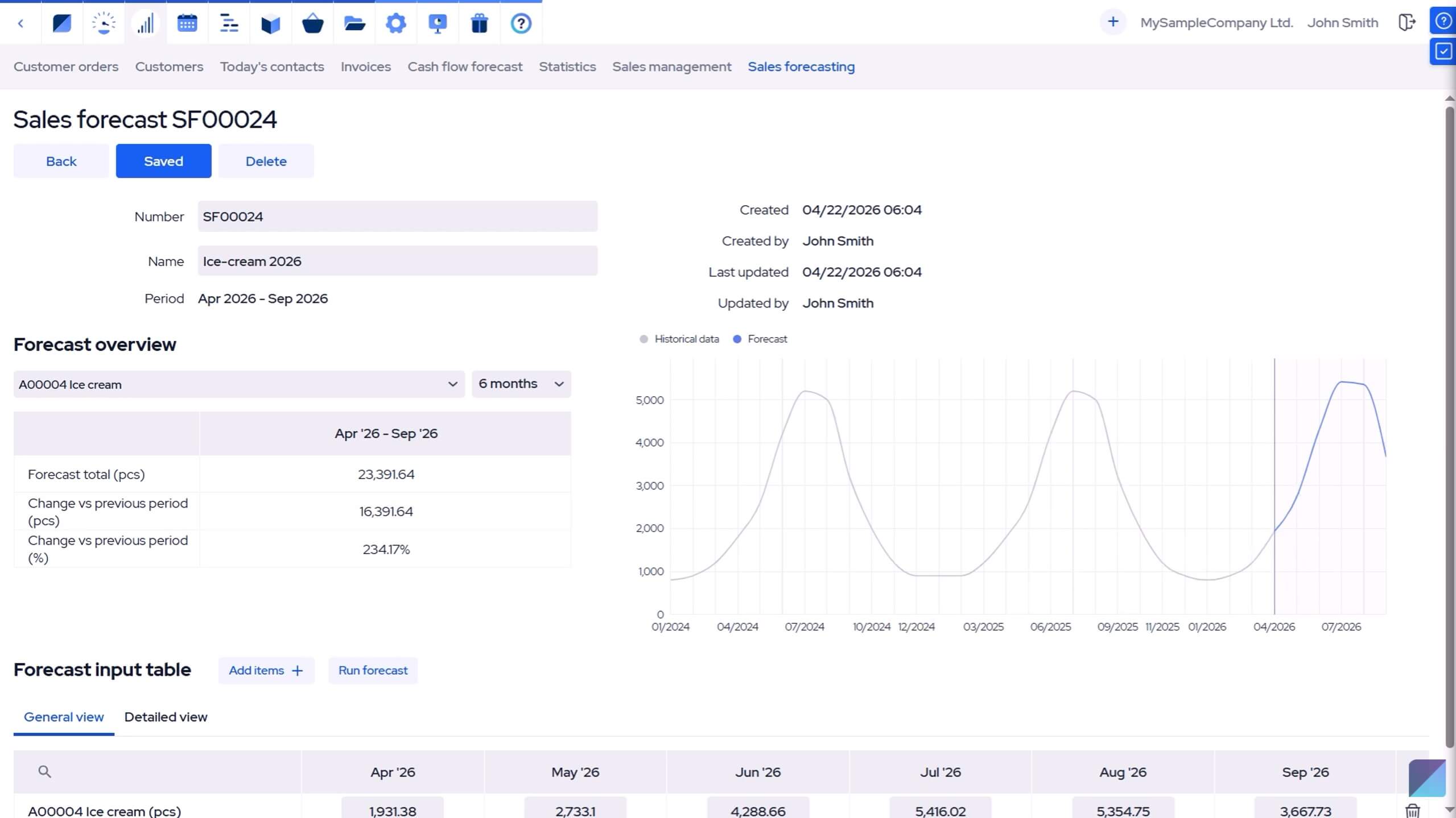
Demand forecasting with a manufacturing ERP system

A manufacturing ERP system connects forecasts with the operational data required to act on them. Instead of forecasting in one system and then rebuilding the plan in another, production software helps planners evaluate expected demand alongside inventory, scheduled production, purchases, and capacity.

From forecast demand to real production plans

As we’ve covered, forecast demand shouldn’t be treated as the confirmed production quantity. A master production schedule combines expected demand with firm customer orders, starting inventory levels, scheduled production, target ending inventory, and planned manufacturing quantities. The resulting plan can then be checked against material requirements and rough-cut capacity.

MRP calculations translate planned finished-product quantities into component and raw-material requirements using bills of materials, current inventory, incoming supply, and lead times. The result is a connected process from expected demand to planned production and purchasing.

Demand forecasting in MRPeasy

MRPeasy provides demand forecasting through its Sales Forecasting functionality. Users can create quantity-based product forecasts for 3-, 6-, 12-, or 18-month horizons using historical customer order data, and manually enter or adjust forecasts when business knowledge needs to be incorporated.

The forecast can be connected with MRPeasy’s Master Production Schedule, where expected sales are considered alongside firm orders, starting inventory, scheduled manufacturing, and planned production jobs.

From there, managers can also review period-based material requirements and workstation-group capacity. This directly connects the demand forecast to manufacturing and procurement planning, rather than leaving it as a standalone prediction.

The system’s automatic forecast feature won’t run without sufficient historical data, and forecasts should still be reviewed against customer knowledge, seasonality, upcoming projects, and other information not present in previous order data.

Frequently asked questions (FAQ)

You might also like: Multi-Level BOM (Indented BOM): Benefits, Tips, and Use Cases